Mosaic plots with `ggplot2`

Haley Jeppson and Heike Hofmann

2025-09-02

Designed to create visualizations of categorical data, geom_mosaic() has the capability to produce bar charts, stacked bar charts, mosaic plots, and double decker plots and therefore offers a wide range of potential plots. The plots below highlight the package’s versatility.

# A few modifications to data
flights <- fly  %>%
  filter(!is.na(do_you_recline), !is.na(rude_to_recline))

bar_examp <- ggplot(data = flights) + 
  geom_mosaic(aes(x=product(do_you_recline), fill = do_you_recline), divider="vbar") +
  theme(axis.text.x = element_blank(),
        axis.ticks.x = element_blank()) +
  labs(y="Do you recline?", x = "", title = "Bar Chart")

spine_examp <- ggplot(data = flights) + 
  geom_mosaic(aes(x=product(do_you_recline), fill = do_you_recline), divider = "vspine") +  
  theme(axis.text.x = element_blank(),
        axis.ticks.x = element_blank()) +
  labs(y="Do you recline?", x = "", title = "Spine Plot")

stackbar_examp <- ggplot(data = flights) + 
  geom_mosaic(aes(x=product(do_you_recline, rude_to_recline), fill = do_you_recline),
              divider=c("vspine", "hbar")) +   
  labs(x="Is it rude to recline?", y = "Do you recline?", title = "Stacked Bar Chart")

mosaic_examp <- ggplot(data = flights) +
  geom_mosaic(aes(x = product(do_you_recline, rude_to_recline), fill = do_you_recline)) +   
  labs(y="Do you recline?", x="Is it rude to recline?", title = "Mosaic Plot (2 variables)") 

mosaic2_examp <- ggplot(data = flights) +
  geom_mosaic(aes(x=product(eliminate_reclining, do_you_recline, rude_to_recline), fill = do_you_recline, alpha = eliminate_reclining)) + 
  scale_alpha_manual(values =c(.7,.9)) +
  theme(axis.text.x = element_text(angle = 90, hjust = 1, vjust = .5)) + 
  labs(y="Do you recline?", x="Eliminate reclining?:Is it rude to recline?", title = "Mosaic Plot (3 variables)")


ddecker_examp <- ggplot(data = flights) +
  geom_mosaic(aes(x=product(do_you_recline, eliminate_reclining, rude_to_recline), fill = do_you_recline, alpha = eliminate_reclining), divider = ddecker()) + 
  scale_alpha_manual(values =c(.7,.9)) +
  theme(axis.text.x = element_text(angle = 90, hjust = 1, vjust = .5)) + 
  labs(y="Do you recline?", x="Eliminate reclining?: Is it rude to recline?", title = "Double Decker Plot")


spine_examp + bar_examp + mosaic_examp + stackbar_examp + mosaic2_examp + ddecker_examp + plot_layout(ncol = 2)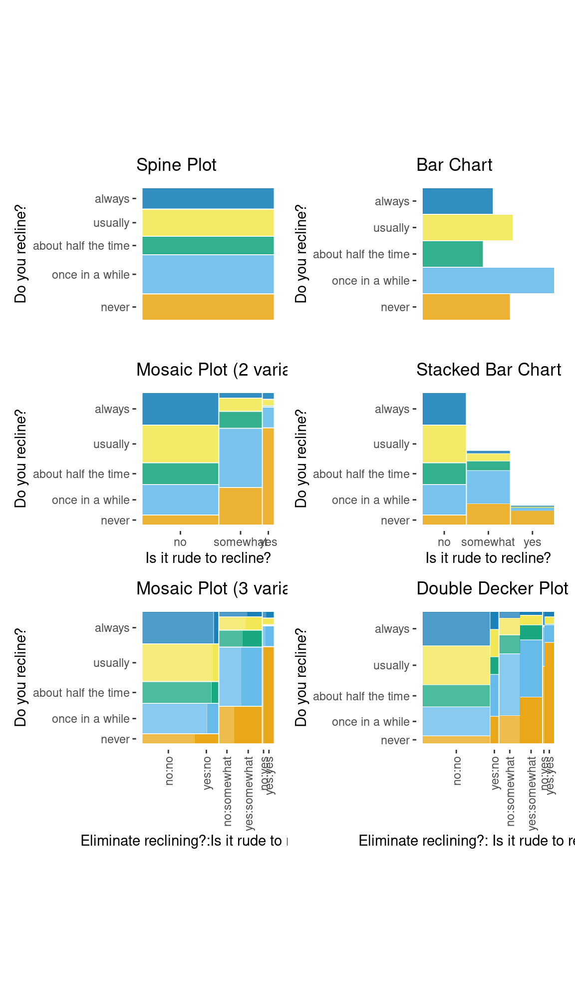

An assortment of plots made with the ggmosaic package.

Furthermore, ggmosaic allows various features to be customized:

• the order of the variables,

• the formula setup of the plot,

• faceting,

• the type of partition, and

• the space between the categories.

How to use ggmosaic

To fit ggmosaic within the ggplot2 framework, we must be able to create the formula from the aesthetics defined in a call. That is, the aesthetics set up the formula which determines how to break down the joint distribution. The main hurdle ggmosaic faced is that mosaic plots do not have a one-to-one mapping between a variable and the x or y axis. To accommodate the variable number of variables, the mapping to x is created by the product() function. For example, the variables var1 and var2 are read in as x = product(var2, var1). The product() function alludes to ggmosaic’s predecessor productplots and to the joint distribution as the product of the conditional and marginal distributions. product() creates a list of the variables and allows for to pass check_aesthetics(), a ggplot2 internal function, and then splits the variables back into a data frame for the calculations.

In geom_mosaic(), the following aesthetics can be specified:

• weight: select a weighting variable

• x: select variables to add to formula

  • declared as x = product(var2, var1, ...)

• alpha: add an alpha transparency to the selected variable

  • unless the variable is called in x, it will be added to the formula in the first position

• fill: select a variable to be filled

  • unless the variable is called in x, it will be added to the formula in the first position after the optional alpha variable.

• conds : select a variable to condition on

  • declared as conds = product(cond1, cond2, ...)

These values are then sent through repurposed productplots functions to create the desired formula: weight ~ alpha + fill + x | conds. Because the plot is constructed hierarchically, the ordering of the variables in the formula is vital.

Examples

One variable

 ggplot(data = flights) +
  geom_mosaic(aes(x = product(rude_to_recline), fill=rude_to_recline)) + 
  labs(title='f(rude_to_recline)')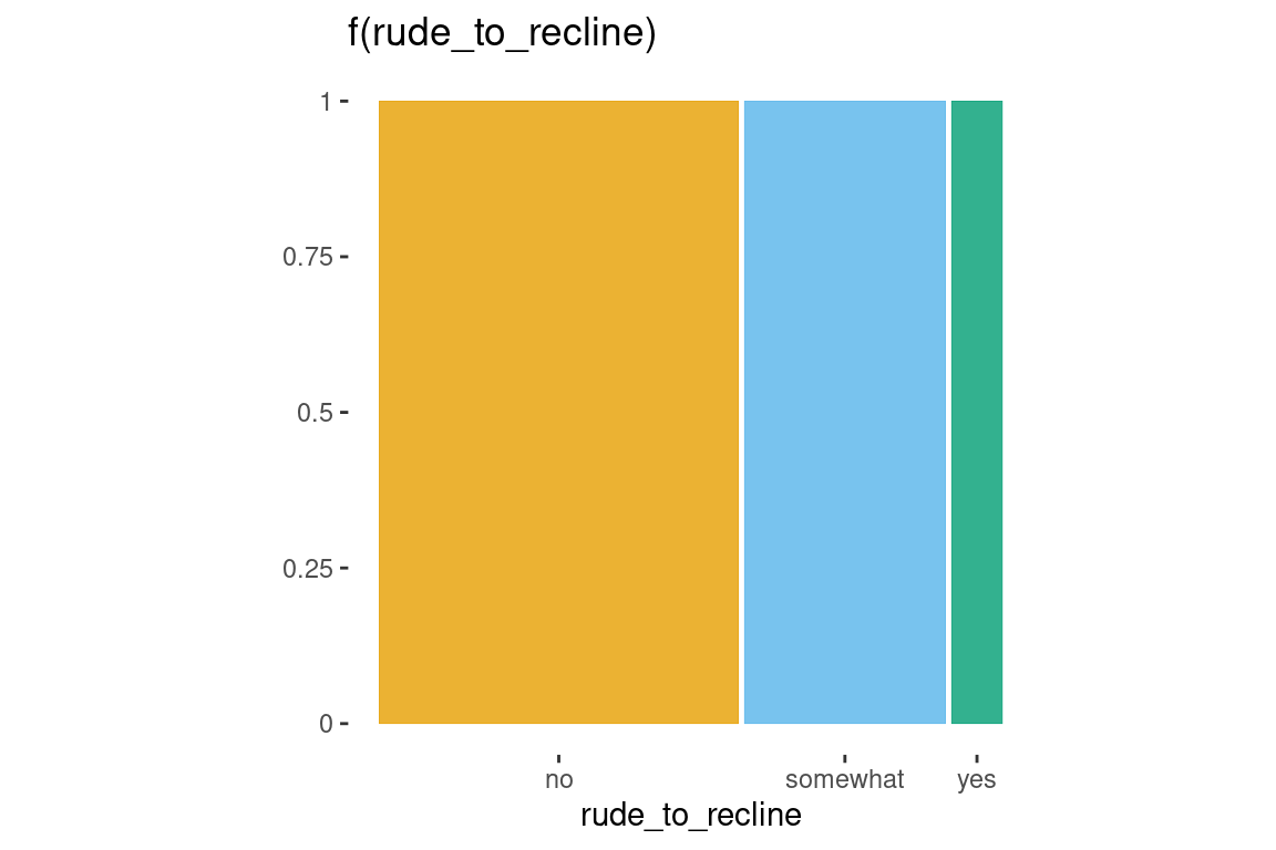

Two variables

ggplot(data = flights) +
  geom_mosaic(aes(x = product(do_you_recline, rude_to_recline), fill=do_you_recline)) + 
  labs(title='f(do_you_recline | rude_to_recline) f(rude_to_recline)')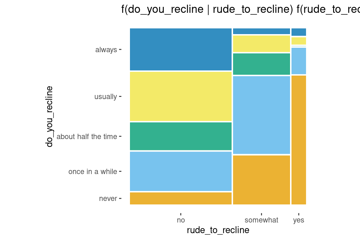

Conditioning

ggplot(data = flights) +
  geom_mosaic(aes(x=product(do_you_recline), fill = do_you_recline, 
                  conds = product(rude_to_recline))) +
  labs(title='f(do_you_recline | rude_to_recline)')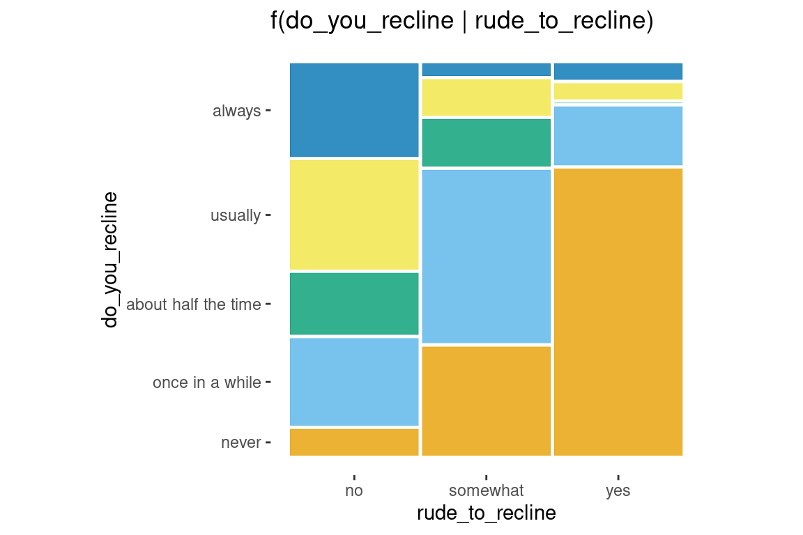

Alternative to conditioning: faceting

ggplot(data = flights) +
  geom_mosaic(aes(x = product(do_you_recline), fill=do_you_recline), divider = "vspine") +
  labs(title='f(do_you_recline | rude_to_recline)') + 
  facet_grid(~rude_to_recline) +
  theme(aspect.ratio = 3,
        axis.text.x = element_blank(),
        axis.ticks.x = element_blank())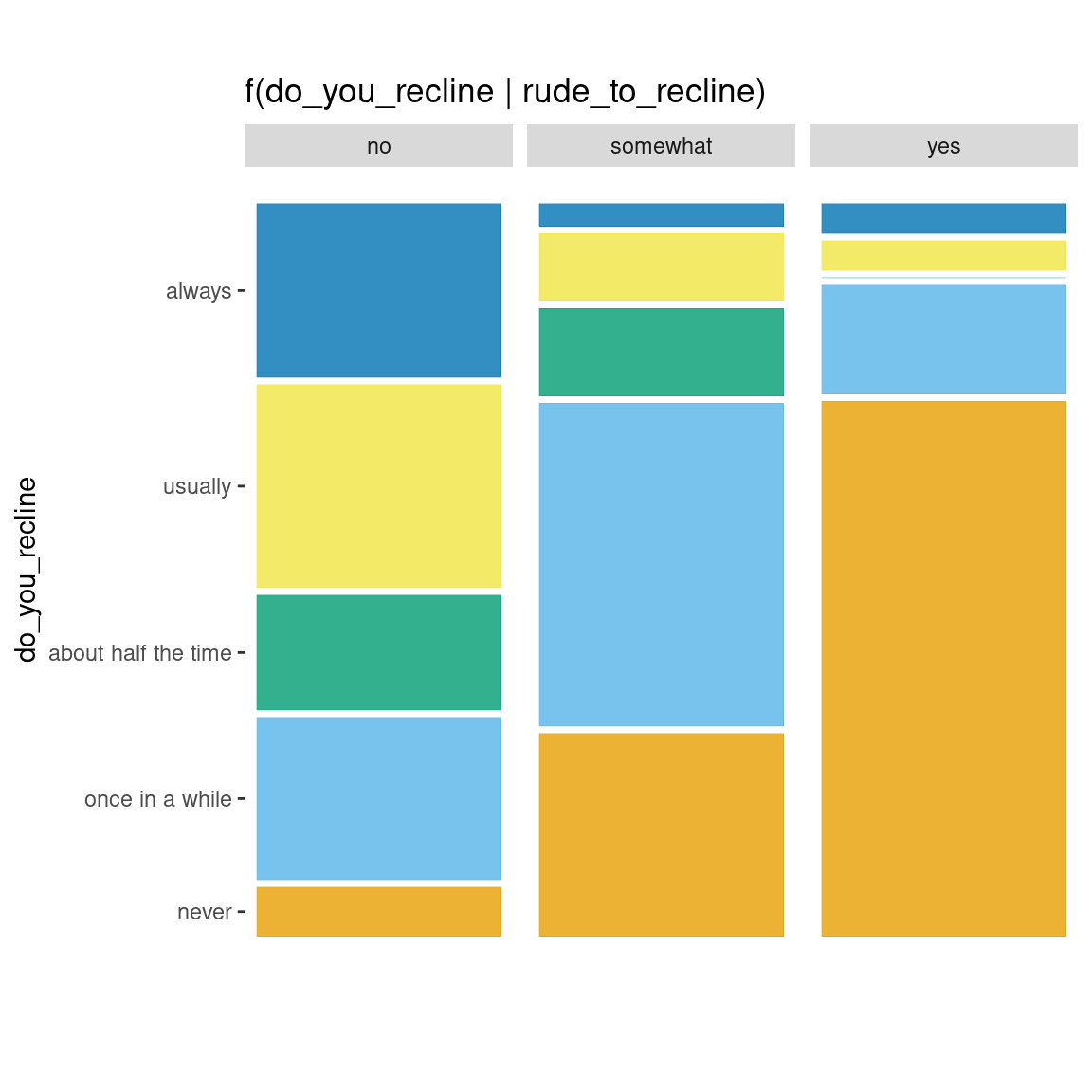

The importance of ordering

order1 <- ggplot(data = flights) +
  geom_mosaic(aes(x = product(do_you_recline, rude_to_recline), fill = do_you_recline)) 

order2 <- ggplot(data = flights) +
  geom_mosaic(aes(x=product(rude_to_recline, do_you_recline), fill = do_you_recline)) 
  
order1 + order2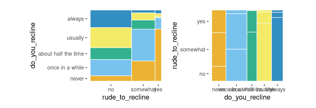

Other features of geom_mosaic()

Arguments unique to geom_mosaic():

• divider: used to declare the type of partitions to be used

• offset: sets the space between the first spine

Divider function: Types of partitioning

Four options available for each partition:

• vspine: width constant, height varies.

• hspine: height constant, width varies.

• vbar: height constant, width varies.

• hbar: width constant, height varies.

part1 <- ggplot(data = flights) + 
  geom_mosaic(aes(x=product(do_you_recline), fill = do_you_recline)) +  
  theme(axis.text = element_blank(),
        axis.ticks = element_blank()) +
  labs(x="", y = "", title = "hspine")

part2 <- ggplot(data = flights) + 
  geom_mosaic(aes(x=product(do_you_recline), fill = do_you_recline),
              divider = "vspine") +  
  theme(axis.text = element_blank(),
        axis.ticks = element_blank()) +
  labs(x="", y = "", title = "vspine")

part3 <- ggplot(data = flights) + 
  geom_mosaic(aes(x=product(do_you_recline), fill = do_you_recline),
              divider = "hbar") +  
  theme(axis.text = element_blank(),
        axis.ticks = element_blank()) +
  labs(x="", y = "", title = "hbar")

part4 <- ggplot(data = flights) + 
  geom_mosaic(aes(x=product(do_you_recline), fill = do_you_recline),
              divider = "vbar") +  
  theme(axis.text = element_blank(),
        axis.ticks = element_blank()) +
  labs(x="", y = "", title = "vbar")

part1 + part2 + part3 + part4 + plot_layout(nrow = 1)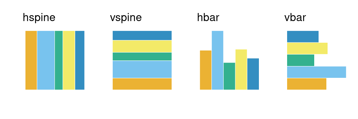

Partitioning with one or more variables

• mosaic()
  • default
  • will use spines in alternating directions
  • begins with a horizontal spine
• mosaic("v")
  • begins with a vertical spine and then alternates
• ddecker()
  • selects n-1 horizontal spines and ends with a vertical spine
• Define each type of partition
  • e.g. c("hspine", "vspine", "hbar")

h_mosaic <- ggplot(data = flights) +
  geom_mosaic(aes(x = product(do_you_recline, rude_to_recline, eliminate_reclining), fill=do_you_recline), divider=mosaic("h")) +
  theme(axis.text=element_blank(), axis.ticks=element_blank()) + 
  labs(x="", y="")

v_mosaic <- ggplot(data = flights) +
  geom_mosaic(aes(x = product(do_you_recline, rude_to_recline, eliminate_reclining), fill=do_you_recline), divider=mosaic("v"))  +
  theme(axis.text=element_blank(), axis.ticks=element_blank()) + 
  labs(x="", y="")

doubledecker <- ggplot(data = flights) +
  geom_mosaic(aes(x = product(rude_to_recline, eliminate_reclining), fill=do_you_recline), divider=ddecker()) +
  theme(axis.text=element_blank(), axis.ticks=element_blank()) + 
  labs(x="", y="")

h_mosaic + v_mosaic + doubledecker + plot_layout(nrow = 1)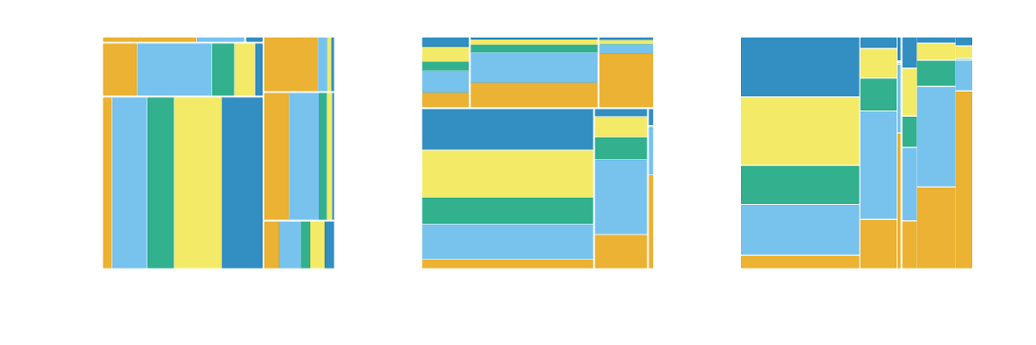

mosaic4 <-  ggplot(data = flights) +
  geom_mosaic(aes(x = product(do_you_recline, rude_to_recline, eliminate_reclining), fill=do_you_recline), divider=c("vspine", "vspine", "hbar"))  +
  theme(axis.text=element_blank(), axis.ticks=element_blank()) + 
  labs(x="", y="")

mosaic5 <-  ggplot(data = flights) +
  geom_mosaic(aes(x = product(do_you_recline, rude_to_recline, eliminate_reclining), fill=do_you_recline), divider=c("hbar", "vspine", "hbar"))  +
  theme(axis.text=element_blank(), axis.ticks=element_blank()) + 
  labs(x="", y="")

mosaic6 <-  ggplot(data = flights) +
  geom_mosaic(aes(x = product(do_you_recline, rude_to_recline, eliminate_reclining), fill=do_you_recline), divider=c("hspine", "hspine", "hspine"))  +
  theme(axis.text=element_blank(), axis.ticks=element_blank()) + 
  labs(x="", y="")

mosaic7 <-  ggplot(data = flights) +
  geom_mosaic(aes(x = product(do_you_recline, rude_to_recline, eliminate_reclining), fill=do_you_recline), divider=c("vspine", "vspine", "vspine"))  +
  theme(axis.text=element_blank(), axis.ticks=element_blank()) + 
  labs(x="", y="")

mosaic4 + mosaic5 + mosaic6 + mosaic7 + plot_layout(nrow = 1)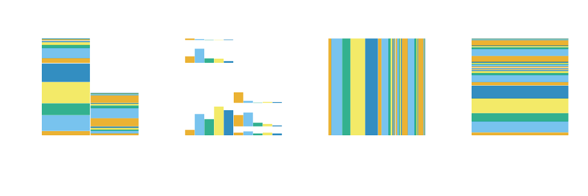

Adjusting the offset

ggmosaic adopts the procedure followed by Hartigan and Kleiner, Friendly, Theus and Lauer, and Hofmann, where an amount of space is allocated for each of the splits, with subsequent divisions receiving a smaller amount of space. The created spaces preserve the impact of small counts. The effect becomes immediately apparent when an empty group is included. In this case, the gaps between the categories, which are empty, create an empty space.

offset: Set the space between the first spine

• default is 0.01

• space between partitions decreases as layers build

offset1 <- ggplot(data = flights) +
  geom_mosaic(aes(x = product(do_you_recline, region), fill=do_you_recline)) + 
  labs(y = "", title=" offset = 0.01") +
  theme(axis.text.y=element_blank(),
        axis.ticks.y=element_blank(),
        axis.text.x = element_text(angle = 90))

offset0 <- ggplot(data = flights) +
  geom_mosaic(aes(x = product(do_you_recline, region), fill=do_you_recline), offset = 0) + 
  labs(y = "", title=" offset = 0") +
  theme(axis.text.y=element_blank(),
        axis.ticks.y=element_blank(),
        axis.text.x = element_text(angle = 90))

offset2 <- ggplot(data = flights) +
  geom_mosaic(aes(x = product(do_you_recline, region), fill=do_you_recline), offset = 0.02) + 
  labs(y="",  title=" offset = 0.02") +
  theme(axis.text.y = element_blank(),
        axis.ticks.y=element_blank(),
        axis.text.x = element_text(angle = 90),
        legend.position = "right")

offset0 + offset1 + offset2 + plot_layout(ncol = 3)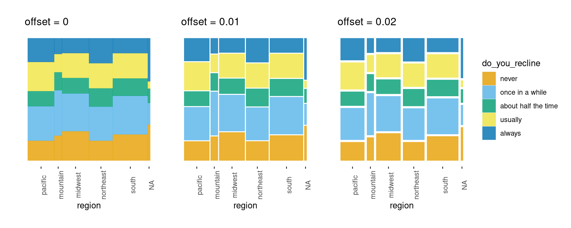

Version compatibility issues with ggplot2

Since the initial release of ggmosaic, ggplot2 has evolved considerably. And as ggplot2 continues to evolve, ggmosaic must continue to evolve alongside it. Although these changes affect the underlying code and not the general usage of ggmosaic, the general user may need to be aware of compatibility issues that can arise between versions. The table below summarizes the compatibility between versions.

ggmosaic	ggplot2	Axis labels	Tick marks
@93e5840	3.3.4	x	x
0.3.3	3.3.3	x	x
0.3.0	3.3.0	x	x
0.2.2	3.3.0	Default labels are okay, but must use scale_*_productlist() to modify	No tick marks
0.2.2	3.2.0	Default labels okay, but must use scale_*_productlist() to modify	x
0.2.0	3.2.0	Default labels are wrong, but can use labs() to modify	x