Chapter 1 An Introduction

Getting Started in R with RStudio

The book is designed for you to follow along in an active way, writing out the examples and experimenting with the code as you go. You will need to install some software first.

R

R is based on the statistical programming language S and can be downloaded for free from www.r-project.org. Currently, to do so, choose: CRAN, then a mirror site in the US, then Download R for Windows, then base, then “Download R 4.2.3 for Windows”. This page also has links to FAQs and other information about R.

R itself is a relatively small application with next to no user interface. Everything works through a command line, or console. At its most basic, you launch it from your Terminal application (on a Mac) or Command Prompt (on Windows) by typing R. Once launched, R awaits your instructions at a command line of its own, denoted by the right angle bracket symbol, >. When you type an instruction and hit return, R interprets it and sends any resulting output back to the console. But although a plain text file and a command line is the absolute minimum you need to work with R, it is a rather spartan arrangement. We can make life easier for ourselves by using RStudio.

RStudio

RStudio is an IDE (integrated development environment), and a convenient interface for R. Think of R as like a car’s engine and RStudio as a car’s dashboard. You can download and install Rstudio from the official Rstudio website. When launched, it starts up an instance of R’s console inside of itself. It also conveniently pulls together various other elements to help you get your work done. These include the document where you are writing your code, the output it produces, and R’s help system. RStudio also knows about RMarkdown, and understands a lot about the R language and the organization of your project.

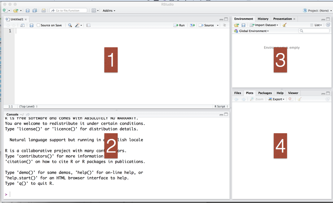
Once you have both R and Rstudio installed, open Rstudio. You should now see four panels: (1) Source editor, (2) Console window, (3) Environment pane, and (4) Other tabs/panes.

Executing code and R script files

You can start coding by typing commands in the Console panel (2). This window is also where the output will appear. For example if you were to type 2+2 and hit return in that window it will return the answer 4.

When using the Console window in RStudio or R, the up and down-arrow on the key-board can be used to scroll through previously entered lines. history() will open a window of previously entered commands (which we’ll see below after entering some). If the font in this R Console is too small, or if you dislike the color or font, you can change it by selecting “Global Options” under the “Tools” menu and clicking on the “Appearance” tab in the pop up window.

Because this Console window is used for so many things it often fills up quickly — and so, if you are doing anything involving a large number of steps, it is often easiest to type them in a script first, which can be viewed in the Source editor (1).

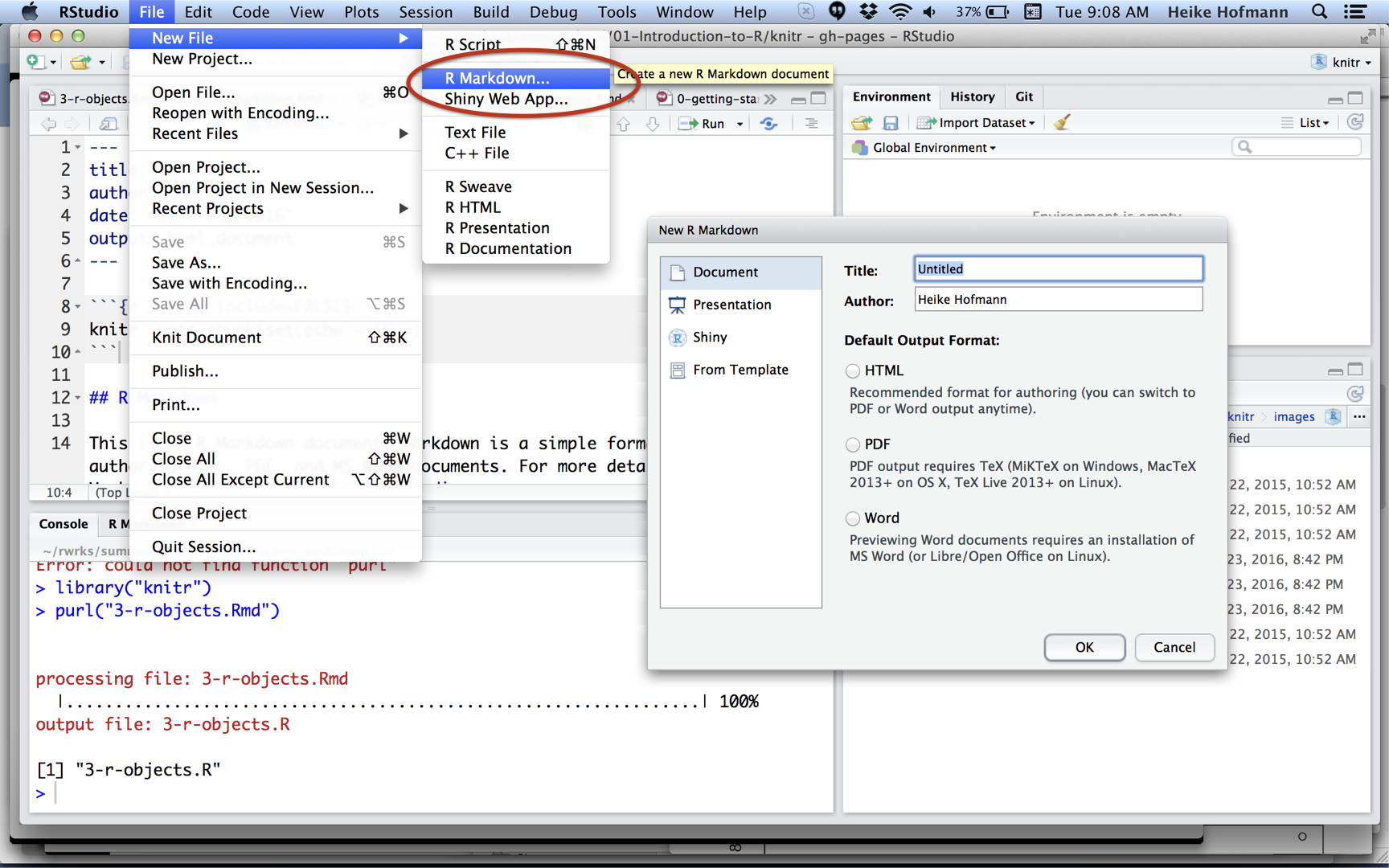
You can create a new script by clicking on the “File” menu and selecting “New File” then “R Script”. A script is a collection of commands that you can save and run again later. To run a command, click in a given line or highlight the text and hit Ctrl+Enter, or click the “Run” button at the top of the script window. You can save your scripts for later use.

1.1 Packages

You’ll also need to install some R packages. An R package is a collection of functions, data, and documentation that extends the capabilities of base R. Using packages is key to the successful use of R. For example, the MASS package contains all of the functions corresponding to the Springer text Modern Applied Statistics with S by Venables and Ripley.

While some of these are automatically included with the basic installation of R, most are not and can installed with the install.packages() function.

install.packages("package_name")

When you run the code to install a package on your own computer, R will download the packages from CRAN and install them on to your computer.

If you have problems installing, make sure that you are connected to the internet, and that https://cloud.r-project.org/ isn’t blocked by your firewall or proxy.

You will not be able to use the functions, objects, and help files in a package until you load it with library().

library(package_name)

The command library() is used to activate a downloaded package and give access to all of its functions and must be done once per session.

Required packages

The remainder of this ebook (and the workshop) requires that you install the tidyverse library and several other add-on packages for R. These libraries provide useful functionality that we will take advantage of throughout the book. You can learn more about the tidyverse’s family of packages at its website.

To install the necessary packages, type the following line of code at R’s command prompt, located in the console window, and hit return.

install.packages("tidyverse")

R should then download and install these packages for you. It may take a little while to download everything.

Once you have installed the tidyverse package, you can load it with the library() function:

library(tidyverse)

1.2 Objects

At the heart of R are the various objects that you enter. An object could be data (in the form of a single value, a vector, a matrix, an array, a list, or a data frame) or a function that you created. Objects are created by assigning a value to the objects name using either <- or =. For example

x <- 3

All R statements where you create objects, assignment statements, have the same form:

object_name <- value

When reading that code say “object name gets value” in your head.

You will make lots of assignments, and <- is a pain to type. You can save time with RStudio’s keyboard shortcut: Alt + - (the minus sign). Notice that RStudio automatically surrounds <- with spaces, which is a good code formatting practice. Code is miserable to read on a good day, so giveyoureyesabreak and use spaces.

If you run x <- 3 in your local console (at the > prompt), R will only give you another prompt. This is because you merely assigned the value; you didn’t ask R to do anything with it. Typing

## [1] 3

will now return the number 3, the value of x. R is case sensitive, so entering X <- 5 will create a separate object:

X <- 5
X

## [1] 5

If you reassign an object, say X <- 7, the original value is over-written:

X <- 7
X

## [1] 7

If you attempt to use the name of a built in function or constant (such as c(), t(), t.test(), or pi()) for one of your variable names, you will likely find that future work you are trying to do gives unexpected results. Notice in the name of t.test() that periods are allowed in names of objects. Other symbols (except numbers and letters) are not allowed.

Your workspace

Note that the up-arrow and history() will now show us the commands we entered previously. This set of all of your created objects (your Workspace) is not saved by default when you exit R, and this is probably a good thing! Attachment to your workspace indicates that you have a non-reproducible workflow. Everything that really matters should be achieved through code that you save in your script, and so any individual R process and the associated workspace is disposable.

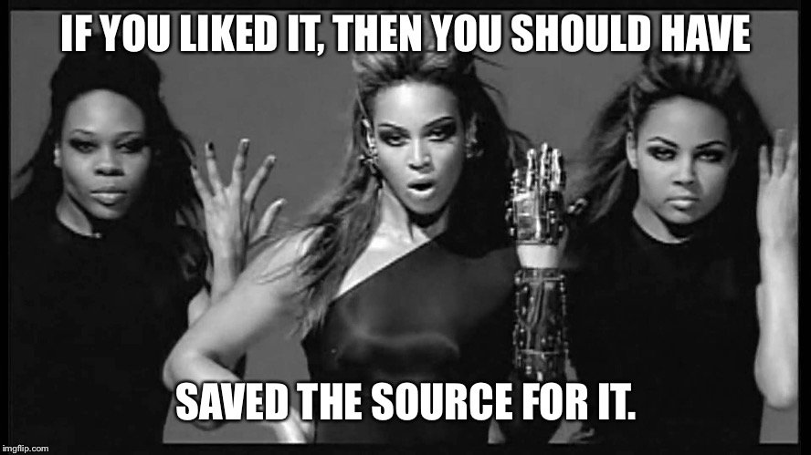
Figure 1.1: Image via Jenny Bryan’s ‘What They Forgot to Teach You About R’

Data types in R

R has a veriety of data types:

logical: boolean values
- ex. TRUE and FALSE
double: floating point numerical values (default numerical type)
- ex. 1.335 and 7
integer: integer numerical values (indicated with an L)
- ex. 7L and 1:3
character: character string
- ex. "hello"
lists: 1d objects that can contain any combination of R objects
& more, but we won’t be focusing on those yet

1.3 Arithmetic and Parentheses

Using R can be a lot like using a calculator. All of the basic arithmetic operations work in R:

X - x

## [1] 4

7 - 3

## [1] 4

will both return the value 4, one by performing the arithmetic on the objects, and the other on the numbers. The other basic mathematical operators are:

+ addition
- subtraction
* multiplication
/ division
^ exponentiation
%*% matrix multiplication

R will often try to do the “common-sense” thing when using arithmetic arguments. For example, if Y is a vector or matrix of values, then Y + 4 will add 4 to each of the values in Y. (So the vector 3, 2, 5 would become 7, 6, 9).

Parentheses work as usual in mathematical statements, but they do not imply multiplication.

X(x+5)

## Error in X(x + 5): could not find function "X"

X*(x+5)

## [1] 56

Notice that the former returns an error about looking for a function called X, while the latter does the arithmetic to return the value 40.

The other use of parentheses in R are to indicate that you attempting to run a function, and, if the function has any options it will contain those. The command:

rnorm(10)

##  [1]  1.8878954  0.6322454  0.7183861  1.4761695  1.2620103  0.7197049
##  [7]  0.5090196 -0.3619615 -0.3187370 -0.4025442

runs the function rnorm() with the argument 10. In this case it is generating a random sample of 10 values from a normal distribution.

1.4 Help!

To see this, we could run the help function on that command.

help(rnorm)

A shortcut, ?rnorm, would also work.

Every help file in R begins with a brief description of the function (or group of functions) in question, followed by all of the possible options (a.k.a. arguments) that you can provide. In this case the value n (the number of observations) is required. Notice that all of the other options are shown as being = some value – this indicates the defaults those values take if you do not enter them. The sample we generated above thus has mean 0 and standard deviation 1.

Below the list of arguments are a brief summary of what the function does (called the Details), a list of the Value (or values) returned by running the function, the Source of the algorithm, and general References on the topic. See Also is often the most useful part of the help for a function as it provides a list of related functions. Finally, there are some Examples that you can cut and paste in to observe the function in action.

1.5 Functions

Functions are (most often) verbs, followed by what they will be applied to in parentheses:

do_this(to_this)
do_that(to_this, to_that, with_those)

It is always safest to enter the values of functions using the names of the arguments:

rnorm(10, sd = 4)

##  [1] -0.3790528  0.7861841 -7.1632380 -1.5314011 -2.0492422  1.5052918
##  [7] -2.3352767  7.3514672 -5.9212688  6.0056887

rather than trusting that the argument you want happens to be first in the list:

rnorm(10, 4)

##  [1] 1.842428 3.014836 5.866371 3.934232 4.188539 5.041615 4.612346 3.349354
##  [9] 4.060865 3.556998

Notice the former puts 4 in for the standard deviation, while the latter is putting it in for the second overall argument, the mean (as seen in the help file).

Note that these values we generated have not been saved as an object, and exist solely on the screen. To save the values we could have assigned the output of our function to an object.

normal.sample <- rnorm(50)
normal.sample

##  [1] -0.657315521 -0.160955273  1.036603648  0.659080126 -0.079563714
##  [6] -0.923549934  1.155224626 -0.958920842  0.774719700 -0.051748151
## [11] -0.033709757  0.331843183 -0.303004359  0.434918033 -2.226721931
## [16]  0.426601807  1.425302785  1.355292522  0.118394199 -0.493144526
## [21] -0.490162834  0.111780677  0.618223767 -0.298698261  0.332890781
## [26] -0.568395526 -0.195307474  0.772448841 -0.898356108 -0.038237328
## [31] -0.429642800 -0.662179395 -0.205809374 -0.906685941  0.619784918
## [36] -1.155524274  0.435646683  0.964037617  0.006933506  0.690698078
## [41] -1.707633203  0.070972828 -1.196988421  0.551246869 -0.719058562
## [46] -0.642679359  1.469032215 -1.217842245  0.225518950  0.256150299

Common statistical functions

A few common statistical functions include:

mean() find the mean
median() find the median
sd() find the standard deviation
var() find the variance
quantile() find the quantiles (percentiles);
- requires the data and the percentile you want
- e.g. quantile(normal.sample, .5) is the median
max() find the maximum
min() find the minimum
summary() find the 5-number summary
hist() construct a histogram
boxplot() construct a boxplot
qqnorm() construct a normal quantile-quantile plot
qqline() add the line to a normal quantile-quantile plot

Trying a few of these out (like mean(normal.sample)) will show us the descriptive statistics and basic graphs for a sample of size 50 from a normal population with mean 0 and standard deviation 1. (Using up arrow can make it quicker to try several in a row.)

As we will see in more detail later, it is possible to create your own functions by using the function function. This one creates a simple measure of skewness.

Skew <- function(x){
    (mean(x) - median(x))/sd(x)}

Note that braces { } in R are used to group several separate commands together, and also occur when using programming commands like loops or if-then statements. They work the same as parentheses in arithmetic expressions.

After entering or new function, it works like any built in function, except that it appears in our objects list.

Skew

## function(x){
##     (mean(x) - median(x))/sd(x)}

Skew()

## Error in mean(x): argument "x" is missing, with no default

Skew(normal.sample)

## [1] -0.01435454

Common mathematical functions

There are also a number of mathematical functions as well. Ones common in statistical applications include:

sqrt() square root
exp() exponent (e to the power)
log() the natural logarithm by default
abs() absolute values
floor() round down
ceiling() round up
round() round to the nearest (even if .5)

1.6 Vectors, Matrices, and Arrays

Vectors

The output from rnorm() is different from the X and x we created as it contains more than just a single value - they are vectors. While we can think of them as vectors in the mathematical sense, we can also think of a vector as simply listing the values of a variable.

Vectors in R are created using the c() function (as in concatonate). Thus,

Y <- c(3, 2, 5)
Y

## [1] 3 2 5

Y + 4

## [1] 7 6 9

Y * 2

## [1]  6  4 10

creates a vector of length three (and we can verify that arithmetic works on it componentwise). Given two vectors arithmetic is also done componentwise:

Z <- c(1, 2, 3)
Y + Z

## [1] 4 4 8

Y * Z

## [1]  3  4 15

Other functions are also evaluated component-wise (if possible):

sqrt(Z)

## [1] 1.000000 1.414214 1.732051

Multiple vectors can be combined together by using the c() function:

YandZ <- c(Y, Z)
YandZ

## [1] 3 2 5 1 2 3

However, when asked to combine vectors of two different types, R will try to force them to be of the same type:

nums <- c(1, 2, 3)
nums

## [1] 1 2 3

lttrs <- c("a", "b", "c")
lttrs

## [1] "a" "b" "c"

c(nums, lttrs)

## [1] "1" "2" "3" "a" "b" "c"

c(nums, lttrs) + 2

## Error in c(nums, lttrs) + 2: non-numeric argument to binary operator

Once we have our desired vector, an element in the vector can be referred to by using square brackets:

YandZ[2]

## [1] 2

YandZ[2:4]

## [1] 2 5 1

YandZ[c(1, 4:6)]

## [1] 3 1 2 3

By using the c() function, and the : to indicate a sequence of numbers, you can quickly refer to the particular portion of the data you are concerned with.

Matrices and arrays

Matrices (two-dimensional) and arrays (more than two dimensions) work similarly - they use brackets to find particular values, and all the values in an array or matrix must be of the same type (e.g. numeric, character, or factor). In the case of matrices, the first values in the brackets indicates the desired rows, and the ones after the comma indicate the desired columns.

Xmat <- matrix(c(3, 2, 5, 1, 2, 3), 
               ncol = 3, byrow = TRUE)
Xmat

##      [,1] [,2] [,3]
## [1,]    3    2    5
## [2,]    1    2    3

Ymat <- rbind(Y, Z)
Ymat

##   [,1] [,2] [,3]
## Y    3    2    5
## Z    1    2    3

Xmat[1, 2:3]

## [1] 2 5

Zmat <- cbind(nums, lttrs)
Zmat

##      nums lttrs
## [1,] "1"  "a"  
## [2,] "2"  "b"  
## [3,] "3"  "c"

In the above code, matrix() is the function to form a vector into a matrix, rbind() places multiple vectors (or matrices) side-by-side as the rows of a new matrix (if the dimensions match), and cbind() does the same for columns.

1.7 Data Frames, Lists, and Attributes

Data frames

In many cases the data set we wish to analyze will not have all of the rows or columns in the same format. This type of data is stored in R as a data frame. A data frame is a rectangular collection of variables (in the columns) and observations (in the rows).

scdata.txt is one such data set, and it can be found in the course materials (its description is found in scdata.pdf). The data can be read in using code similar to the below (assuming a similar file structure).

url <- "https://people.stat.sc.edu/habing/RforQM/scdata.txt"
sctable <- readr::read_table(url)

The function read_table() reads in our file as a tibble, unlike read.table() which reads in the file as R’s traditional data.table. Tibbles are data frames, but more opinionated, and they tweak some older behaviors to make working in the tidyverse a little easier.

There are a few good reasons to favor {readr} functions over the base equivalents:

They are typically much faster than their base equivalents. Long running jobs have a progress bar, so you can see what’s happening. If you’re looking for raw speed, try data.table::fread(). It doesn’t fit quite so well into the tidyverse, but it can be quite a bit faster.
They produce tibbles, they don’t convert character vectors to factors, use row names, or munge the column names. These are common sources of frustration with the base R functions.
They are more reproducible. Base R functions inherit some behavior from your operating system and environment variables, so import code that works on your computer might not work on someone else’s.
Tibbles are designed so that you don’t accidentally overwhelm your console when you print large data frames.

Some older functions don’t work with tibbles. If you encounter one of these functions, use as.data.frame() to turn a tibble back to a data.frame. The main reason that some older functions don’t work with tibble is the [ function. With base R data frames, [ sometimes returns a data frame, and sometimes returns a vector. With tibbles, [ always returns another tibble.

Inspecting objects

To inspect the data without needing to print out the entire data set, we can try out the following commands:

head()
tail()
summary()
str()
dim()

For example, use head() and tail() to see the first and last rows. This lets you check the variable names as well as the number of observations successfully read in.

head(sctable)

## # A tibble: 6 × 27
##   County Region Births Death InfMort Minor…¹ Over65 PopChng PopDens Urban Income
##   <chr>  <chr>   <dbl> <dbl>   <dbl>   <dbl>  <dbl>   <dbl>   <dbl> <dbl>  <dbl>
## 1 Abbev… Upsta…   12.5  10.3    15.1    31.7   14.7     9.7    51.5  23.4  32635
## 2 Aiken  Midla…   12.1   9.8     9.6    28.6   12.8    17.8   133.   60.9  37889
## 3 Allen… LowCo…   14.8  12.1    18.5    72.6   12.7    -4.4    27.5  59    20898
## 4 Ander… Upsta…   13    10.7    10.3    18.4   13.7    14.2   231.   58.3  36807
## 5 Bambe… Midla…   11.5   9.9    21.7    63.5   13.9    -1.4    42.4  45.7  24007
## 6 Barnw… Midla…   14    10.9    21.4    44.8   12.6    15.7    42.8  14.9  28591
## # … with 16 more variables: ConsInc <dbl>, FarmInc <dbl>, ManIncom <dbl>,
## #   RetInc <dbl>, FdStmps <dbl>, MoblHms <dbl>, NoCar <dbl>, PlumProb <dbl>,
## #   PoorChild <dbl>, Unemp <dbl>, Coll4 <dbl>, Crime <dbl>, HSGrad <dbl>,
## #   JuvDel <dbl>, MVDeath <dbl>, SchlSpnd <dbl>, and abbreviated variable name
## #   ¹Minority

tail(sctable)

## # A tibble: 6 × 27
##   County Region Births Death InfMort Minor…¹ Over65 PopChng PopDens Urban Income
##   <chr>  <chr>   <dbl> <dbl>   <dbl>   <dbl>  <dbl>   <dbl>   <dbl> <dbl>  <dbl>
## 1 Saluda Midla…   11.2  11.3     4.7    34.2   14.5    16.7    42.5  18.7  35774
## 2 Spart… Upsta…   13.1   9.8     7.9    24.9   12.5    11.9   313.   64.8  37579
## 3 Sumter Midla…   15.6   8.9     8.5    50     11.2     3.3   157.   62.1  33278
## 4 Union  Upsta…   10.7  13.2    12.8    32.2   15.6    -1.5    58.1  35.7  31441
## 5 Willi… Peedee   12.6  11.8     8.8    67.3   13       1.1    39.8  15.1  24214
## 6 York   Upsta…   13.4   7.7     7.6    22.7   10.4    25.2   241.   64.3  44539
## # … with 16 more variables: ConsInc <dbl>, FarmInc <dbl>, ManIncom <dbl>,
## #   RetInc <dbl>, FdStmps <dbl>, MoblHms <dbl>, NoCar <dbl>, PlumProb <dbl>,
## #   PoorChild <dbl>, Unemp <dbl>, Coll4 <dbl>, Crime <dbl>, HSGrad <dbl>,
## #   JuvDel <dbl>, MVDeath <dbl>, SchlSpnd <dbl>, and abbreviated variable name
## #   ¹Minority

Extracting parts of objects

For object x, we can extract parts in the following manner (rows and columns are vectors of indices):

x$variable
x[, "variable"]
x[rows, columns]
x[1:5, 2:3]
x[c(1,5,6), c("County", "Region")]
x$variable[rows]

Many of these extraction methods access the rows and columns of a data frame by treating it similarly to a matrix:

County1 <- sctable[1, ]
Birth.Death <- sctable[ , 3:4]

This simplicity sometimes causes trouble though. While Birth.Death may look on the screen like it is a matrix, it is still a data frame and many functions which use matrix operations (like matrix multiplication) will give an error. The attributes() function will show us the true status of our object (it returns NULL for a numeric vector and the dimensions if a matrix):

Birth.Death

## # A tibble: 46 × 2
##    Births Death
##     <dbl> <dbl>
##  1   12.5  10.3
##  2   12.1   9.8
##  3   14.8  12.1
##  4   13    10.7
##  5   11.5   9.9
##  6   14    10.9
##  7   15.8   7.8
##  8   14.4   6.6
##  9   11.5  11.1
## 10   14.5   8.5
## # … with 36 more rows

attributes(Birth.Death)

## $names
## [1] "Births" "Death" 
## 
## $row.names
##  [1]  1  2  3  4  5  6  7  8  9 10 11 12 13 14 15 16 17 18 19 20 21 22 23 24 25
## [26] 26 27 28 29 30 31 32 33 34 35 36 37 38 39 40 41 42 43 44 45 46
## 
## $class
## [1] "tbl_df"     "tbl"        "data.frame"

BD.matrix <- as.matrix(Birth.Death)
attributes(BD.matrix)

## $dim
## [1] 46  2
## 
## $dimnames
## $dimnames[[1]]
## NULL
## 
## $dimnames[[2]]
## [1] "Births" "Death"

The $ is used to access whatever corresponds to an entry in the names attribute:

Birth.Death$Births

##  [1] 12.5 12.1 14.8 13.0 11.5 14.0 15.8 14.4 11.5 14.5 13.3 12.3 12.1 12.3 13.0
## [16] 12.4 15.6 12.9 10.3 12.8 15.3 12.7 14.0 12.6 13.9 12.7 14.3 12.8 12.2 11.6
## [31] 12.9 14.0  7.6 13.8 11.9 12.5 11.7 13.8 11.2 13.3 11.2 13.1 15.6 10.7 12.6
## [46] 13.4

This is particularly useful when trying to access a portion of the output of a function for later use. For example, later we will see a method of doing statistical inference called the t-test. In R, this is performed by the function t.test() which can create a great deal of output on the screen.

t.test(normal.sample)

## 
##  One Sample t-test
## 
## data:  normal.sample
## t = -0.41638, df = 49, p-value = 0.679
## alternative hypothesis: true mean is not equal to 0
## 95 percent confidence interval:
##  -0.2771565  0.1820170
## sample estimates:
##   mean of x 
## -0.04756977

If you only want the part called the “p-value” for later use we can pull that out of the output.

t.out <- t.test(normal.sample)
attributes(t.out)

## $names
##  [1] "statistic"   "parameter"   "p.value"     "conf.int"    "estimate"   
##  [6] "null.value"  "stderr"      "alternative" "method"      "data.name"  
## 
## $class
## [1] "htest"

t.out$p.value

## [1] 0.6789512

We could then save the resulting value as part of a vector or matrix of other p-values, for example.

The $ is also used to access named parts of lists, which we will see can be used to store a variety of kinds of information in a single object.

1.8 RMarkdown

Beyond data analysis, coding, and creating graphics, R and RStudio also allow for the creation of documents using Markdown. Markdown is a particular type of markup language. Markup languages are designed to produce documents from plain text. Some of you may be familiar with LaTeX, another (less human friendly) markup language for creating pdf documents. LaTeX gives you much greater control, but it is restricted to pdf and has a much greater learning curve.

Markdown is becoming a standard and many websites will generate HTML from Markdown (e.g. GitHub, Stack Overflow, reddit, …). It is also relatively easy:

*italic*
**bold**
# Header 1
## Header 2
### Header 3
- List item 1
- List item 2
    - item 2a
    - item 2b
1. Numbered list item 1
1. Numbered list item 2
    - item 2a
    - item 2b

Have a look at RStudio’s RMarkdown cheat sheet.

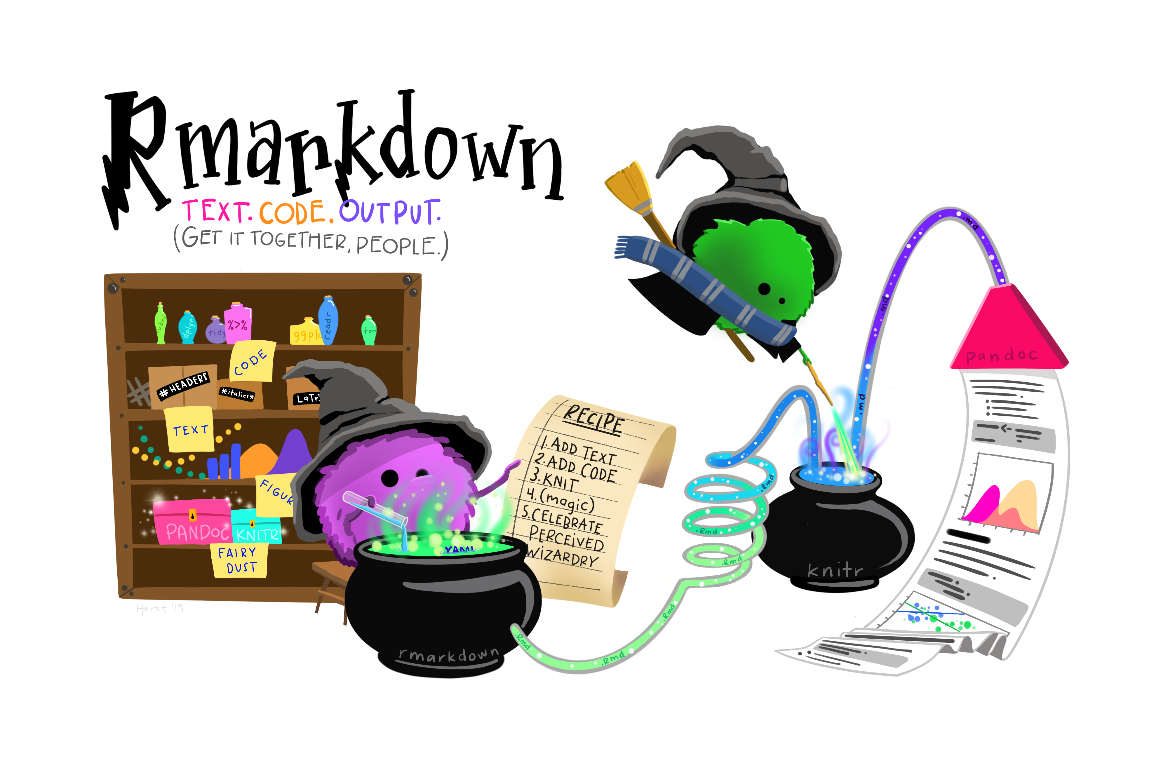
Figure 1.2: Artwork by allison horst

RMarkdown is an authoring format that enables easy creation of dynamic documents, presentations, and reports from R. It combines markdown syntax with embedded R code chunks that are run so their output can be included in the final document.

Most importantly, RMarkdown creates fully reproducible reports since each time you knit the analysis is run from the beginning, encouraging transparency. Collaborators (including your future self) will thank you for integrating your analysis and report.

For a more in depth introduction, see Getting Started with R Markdown — Guide and Cheatsheet, and to expand on your introduction, see R Markdown tips, tricks, and shortcuts.

Exercise: Create your first Rmarkdown.

Open RStudio, create a new project.
Create a new RMarkdown file and knit it.
Make changes to the markdown formatting and knit again (use the RMarkdown cheat sheet)
If you feel adventurous, change some of the R code and knit again.