class: center, middle, inverse, title-slide .title[ # Advanced Customization ] --- background-image: url(https://raw.githubusercontent.com/allisonhorst/stats-illustrations/master/rstats-artwork/ggplot2_masterpiece.png) background-size: 450px background-position: 50% 70% ## Graphics for communication We have mostly been focused on **exploratory data analysis** - i.e., used plots as tools for exploration After you understand your data, you need to **communicate** your understanding to others. <br/><br/><br/><br/><br/><br/><br/><br/><br/> <br/><br/><br/> <p style="font-size:15px;text-align:center;">Artwork by <a href="https://twitter.com/allison_horst?ref_src=twsrc%5Egoogle%7Ctwcamp%5Eserp%7Ctwgr%5Eauthor">@allison_horst</a></p> --- ## `{ggplot2}` provides defaults ... <br/> - but every aspect of the plot can be changed - colors are controlled through **scales** - **themes** control presentation of non-data elements --- class: inverse ## Outline <br> ### 1. labels & annotations ### 2. `{ggplot2}` scales ### 3. scales & color choices ### 4. themes --- ## Adding labels You add labels with the `labs()` function. - Labels that can be modified include: - `x` - `y` - `title` - `subtitle` - `caption` - `color` <br> Other methods of modifying labels: - `ggtitle(main, subtitle)`: plot title & subtitle - `xlab()`, `ylab()`: axes titles --- ## Adding labels ```r ggplot(mpg, aes(displ, hwy)) + geom_point(aes(color = class)) + labs(title = "Fuel efficiency generally decreases with engine size", subtitle = "Two seaters (sports cars) are an exception because of their light weight", caption = "Data from fueleconomy.gov", x = "Engine displacement (L)", y = "Highway fuel economy (mpg)", colour = "Car type") ``` <!-- --> --- ## Adding text Create a subset of the data using `{dplyr}` containing the most efficient car in each class .left-code[ ```r best_in_class <- mpg %>% group_by(class) %>% filter(row_number(desc(hwy)) == 1) best_in_class ``` ] .right-plot[ ``` ## # A tibble: 7 × 11 ## # Groups: class [7] ## manufacturer model displ year cyl trans drv cty hwy fl class ## <chr> <chr> <dbl> <int> <int> <chr> <chr> <int> <int> <chr> <chr> ## 1 chevrolet corvette 5.7 1999 8 manu… r 16 26 p 2sea… ## 2 dodge caravan 2wd 2.4 1999 4 auto… f 18 24 r mini… ## 3 nissan altima 2.5 2008 4 manu… f 23 32 r mids… ## 4 subaru forester a… 2.5 2008 4 manu… 4 20 27 r suv ## 5 toyota toyota tac… 2.7 2008 4 manu… 4 17 22 r pick… ## 6 volkswagen jetta 1.9 1999 4 manu… f 33 44 d comp… ## 7 volkswagen new beetle 1.9 1999 4 manu… f 35 44 d subc… ``` ] --- ## Adding text Use `geom_text()` or `geom_label()` to label interesting observations. .left-code[ ```r best_in_class <- mpg %>% group_by(class) %>% filter(row_number(desc(hwy)) == 1) ggplot(mpg, aes(displ, hwy)) + geom_point(aes(colour = class)) + * geom_text(data = best_in_class, * aes(label = model)) ``` ] .right-plot[ <img src="advanced-customization_files/figure-html/unnamed-chunk-5-1.png" width="100%" /> ] --- ## Adding text Use `geom_label()` (or even better, use `ggrepel::geom_label_repel()`) for increased readability .left-code[ ```r ggplot(mpg, aes(displ, hwy)) + geom_point(aes(colour = class)) + geom_point(data = best_in_class, size = 3, shape = 1) + * ggrepel::geom_label_repel( * data = best_in_class, * aes(label = model)) ``` ] .right-plot[ <img src="advanced-customization_files/figure-html/unnamed-chunk-6-1.png" width="100%" /> ] --- ## Adding text Make use of `stat`s and `after_stat()` for placement .left-code[ ```r ggplot(mpg, aes(class)) + geom_bar() + * geom_text( * aes( * y = after_stat(count + 2), * label = after_stat(count) * ), * stat = "count" * ) ``` ] .right-plot[ <img src="advanced-customization_files/figure-html/unnamed-chunk-7-1.png" width="100%" /> ] --- ## Annotations An **annotation** is a separate layer that doesn't connect to other elements in the plot and is used to add fixed elements to a data visualization The `annotate()` function creates an annotation layer - arguments include `geom`, and positions (`x`, `y`, `xmin`, `ymin`, etc.) --- ## Example ```r p <- ggplot(mpg, aes(displ, hwy)) + geom_point(data = dplyr::filter(mpg, manufacturer == "subaru"), colour = "orange", size = 3) + geom_point() p ``` <!-- --> --- ## Adding annotations ```r p + annotate(geom = "curve", x = 4, y = 35, xend = 2.65, yend = 27, curvature = .3, arrow = arrow(length = unit(2, "mm"))) + annotate(geom = "text", x = 4.1, y = 35, label = "subaru", hjust = "left") ``` <!-- --> --- class: yourturn .center[ ## Your Turn ] ### Annotate this plot by adding a reference line with `geom_abline()`<br>&emsp;- Modify the color or size of the line. ```r library(NCME23data) ggplot(pisa_usa, aes(x = math, y = reading)) + geom_point(color = "#3C5488", alpha = .7) ``` --- class: inverse, middle, center # Scales --- ## Scales **Recall**: Scales control the details of how data values are translated to visual properties. - Every aes value has a corresponding family of scales functions - `scale_{aes}_*()`, e.g. `scale_x_continuous()` - Values of the `*` depend on the aes - These scale functions have many arguments including: - `name`: label of the axis/legend - `breaks`: numeric positions of breaks on axes/legends - `labels`: labels of the breaks on axes/legends - `limits`: continuous axis limits - `expand`: padding around data - `na.value`: what to do with missings - `trans`: continuous transformations of data - `guide`: function to create guide/legend - `date_breaks`: breaks for date variables --- ## Scales for axes .pull-left[ `scale_x_*()`, `scale_y_*()` - continuous - discrete - binned - log10 - sqrt - date - datetime - reverse ] .pull-right[ ] --- ## Scales for axes .left-code[ ```r p ``` ] .right-plot[ <img src="advanced-customization_files/figure-html/unnamed-chunk-12-1.png" width="100%" /> ] --- ## Scales for axes .left-code[ ```r p + * scale_x_continuous() ``` ] .right-plot[ <img src="advanced-customization_files/figure-html/unnamed-chunk-13-1.png" width="100%" /> ] --- ## Scales for axes .left-code[ ```r p + scale_x_continuous( * "Engine displacement, in litres", * breaks = c(2,4,6) ) ``` ] .right-plot[ <img src="advanced-customization_files/figure-html/unnamed-chunk-14-1.png" width="100%" /> ] --- ## Scales for color - Colors are controlled through scales - `scale_colour_discrete` (`scale_colour_hue`) and `scale_colour_continuous` (`scale_colour_gradient`) are the default choices for factor variables and numeric variables - we can change parameters of the default scale, or we can change the scale function .pull-left[ `scale_color_*()`, `scale_fill_*()` - manual - continuous - brewer/distiller/fermenter - gradient/gradient2/gradientn - steps - viridis ] --- ## Continuous color scales Default continuous colour scheme .left-code[ ```r ggplot(mpg, aes(x = displ, y = hwy)) + geom_point(aes(color = cyl)) ``` ] .right-plot[ <img src="advanced-customization_files/figure-html/unnamed-chunk-15-1.png" width="100%" /> ] --- ## Continuous color scales Default continuous colour scheme .left-code[ ```r ggplot(mpg, aes(x = displ, y = hwy)) + geom_point(aes(color = cyl)) + * scale_colour_continuous() ``` ] .right-plot[ <img src="advanced-customization_files/figure-html/unnamed-chunk-16-1.png" width="100%" /> ] --- ## Discrete color scales Default discrete colour scheme .left-code[ ```r ggplot(mpg, aes(x = displ, y = hwy)) + geom_point( aes(color = factor(cyl)) ) ``` ] .right-plot[ <img src="advanced-customization_files/figure-html/unnamed-chunk-17-1.png" width="100%" /> ] --- ## Discrete color scales Default discrete colour scheme .left-code[ ```r ggplot(mpg, aes(x = displ, y = hwy)) + geom_point( aes(color = factor(cyl)) ) + * scale_colour_discrete() ``` ] .right-plot[ <img src="advanced-customization_files/figure-html/unnamed-chunk-18-1.png" width="100%" /> ] --- ## Color & Fill Area geoms (barcharts, histograms, polygons) use `fill` to map values to the fill color - only discrete color scales can be used e.g. `scale_fill_brewer` - most general: `scale_fill_manual(..., values)` - `values` is a vector of color values. - at least as many colors as levels in the variable have to be listed <br> **Color Values**: - can be defined as a hex value or a name of a color - [R colors pdf](http://www.stat.columbia.edu/~tzheng/files/Rcolor.pdf) --- ## Manual color scales .left-code[ ```r ggplot(mpg, aes(x = displ, y = hwy, color = factor(cyl) )) + geom_point() + * scale_color_manual( * "cylinders", * values = c( * "turquoise3", "magenta", * "mediumpurple4", "orange" * ) * ) ``` ] .right-plot[ <img src="advanced-customization_files/figure-html/unnamed-chunk-19-1.png" width="100%" /> ] --- background-image: url(https://www.datanovia.com/en/wp-content/uploads/dn-tutorials/ggplot2/figures/030-ggplot-colors-wes-anderson-color-palettes-r-1.png) background-size: 325px background-position: 85% 55% ## Predefined color palettes .tall[ .pull-left[ The most commonly used color scales, include: - Okabe-Ito palette [[ggokabeito package](https://malcolmbarrett.github.io/ggokabeito/)] - Viridis color scales <br>[[viridis package](https://cran.r-project.org/web/packages/viridis/vignettes/intro-to-viridis.html)] - Colorbrewer palettes [[RColorBrewer package](http://colorbrewer2.org/)] - Scientific journal color palettes [[ggsci package](https://cran.r-project.org/web/packages/ggsci/vignettes/ggsci.html)] - Wes Anderson color palettes [[wesanderson package](https://github.com/karthik/wesanderson/blob/master/README.md)] <br/> For the most extensive list I've found, look [here](https://github.com/EmilHvitfeldt/r-color-palettes) ] ] --- ## Other color scales While function name is predictable, arguments are not .left-code[ ```r ggplot(mpg, aes(x = displ, y = hwy, color = factor(cyl) )) + geom_point() + * scale_colour_brewer( * palette = 'Dark2' * ) ``` ] .right-plot[ <img src="advanced-customization_files/figure-html/unnamed-chunk-20-1.png" width="100%" /> ] --- ## Legends The **guide** or **legend** connects non-axis aesthetics in the data visualization like color and size to the data The `guides()` function controls all legends by connecting to the aes. - `guide_colorbar()`: continuous colors - `guide_legend()`: discrete values (shapes, colors) - `guide_axis()`: control axis text/spacing, add a secondary axis - `guide_bins()`: creates "bins" of values in the legend - `guide_colorsteps()`: makes colorbar discrete --- ## Guides .left-code[ ```r ggplot(mpg, aes(x = displ, y = hwy, color = cyl )) + geom_point() + * scale_color_gradientn( * "cylinders", * colours = c( * "#6C5B7B", "#C06C84", * "#F67280", "#F8B195" * ) * ) ``` ] .right-plot[ <img src="advanced-customization_files/figure-html/unnamed-chunk-21-1.png" width="100%" /> ] --- ## Guides .left-code[ ```r ggplot(mpg, aes(x = displ, y = hwy, color = cyl )) + geom_point() + scale_color_gradientn( "cylinders", colours = c( "#6C5B7B", "#C06C84", "#F67280", "#F8B195" ), * guide = guide_colorsteps( * barwidth = 0.5, * barheight = 8 * ) ) ``` ] .right-plot[ <img src="advanced-customization_files/figure-html/unnamed-chunk-22-1.png" width="100%" /> ] --- ## Guides .left-code[ ```r ggplot(mpg, aes(y = class, fill = class )) + geom_bar() + ggokabeito::scale_fill_okabe_ito() ``` ] .right-plot[ <img src="advanced-customization_files/figure-html/unnamed-chunk-23-1.png" width="100%" /> ] --- ## Guides .left-code[ ```r ggplot(mpg, aes(y = class, fill = class )) + geom_bar() + ggokabeito::scale_fill_okabe_ito( * guide = guide_legend( * reverse = TRUE * ) ) ``` ] .right-plot[ <img src="advanced-customization_files/figure-html/unnamed-chunk-24-1.png" width="100%" /> ] --- class: inverse, middle, center # Themes --- ## Themes The **theme** describes the appearance of the plot, such as the background color, font size, positions of labels, etc. <br> Specific themes: - `theme_grey()`: default - `theme_bw()`: white background, gray gridlines - `theme_classic()`: looks more like base R plots - `theme_void()`: removes all background elements, all axes elements, keeps legends <br/> In addition to `{ggplot2}`’s built-in themes, other packages like `{ggthemes}` allow you to choose from even more styles. --- ## Theme examples ```r p <- ggplot(mpg, aes(x = displ, y = cty, colour= factor(class))) + geom_point() ``` .tall[ .pull-left[ ```r p + theme_grey() ``` <!-- --> ] .pull-right[ ```r p + theme_minimal() ``` 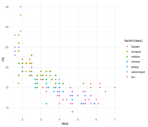<!-- --> ] ] --- ## Theme examples ```r p <- ggplot(mpg, aes(x = displ, y = cty, colour= factor(class))) + geom_point() ``` .tall[ .pull-left[ ```r p + theme_light() ``` 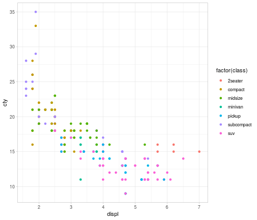<!-- --> ] .pull-right[ ```r p + theme_dark() ``` 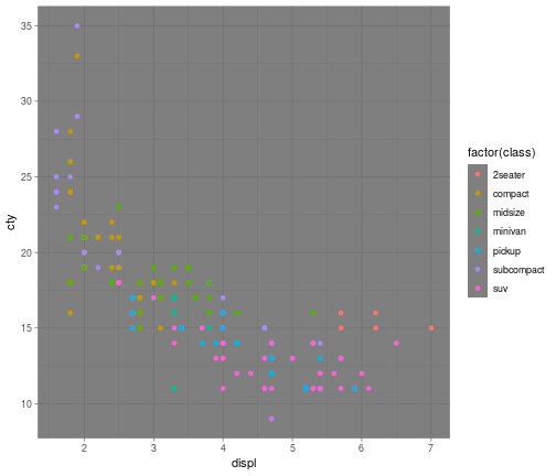<!-- --> ]] --- ## More themes ```r library(ggthemes) ``` .tall[ .pull-left[ ```r p + theme_excel() ``` 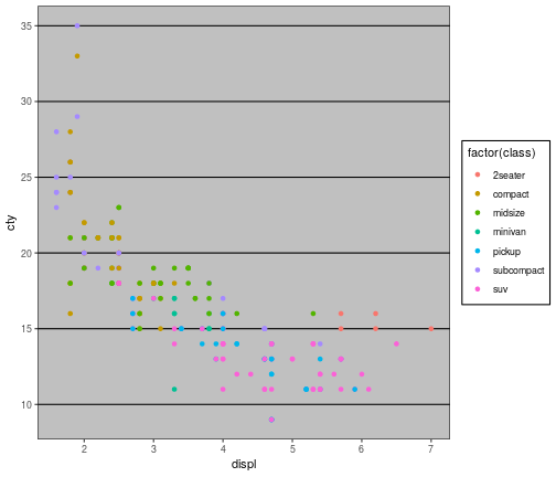<!-- --> ] .pull-right[ ```r p + theme_fivethirtyeight() ``` <!-- --> ]] --- ## Theme customization The `theme()` function can modify any non-data element of the plot. - adjust the appearance of every "non-data element" of the viz - fonts, background, text positioning, legend appearance, facet appearance, etc. <br> **Rule of thumb**: when changing an element that shows data, use `aes()` and scales. Otherwise, use themes. --- ## Elements of themes - **Line elements**: axis lines, minor and major grid lines, plot panel border, axis ticks background color, etc. - **Text elements**: plot title, axis titles, legend title and text, axis tick mark labels, etc. - **Rectangle elements**: plot background, panel background, legend background, etc. <br/> There is a specific function to modify each of these three elements : - `element_line()` to modify the line elements of the theme - `element_text()` to modify the text elements - `element_rect()` to change the appearance of the rectangle elements - `element_blank()` to draw nothing and assign no space --- ## Elements of themes - Axis: `axis.line`, `axis.text.x`, `axis.text.y`, `axis.ticks`, `axis.title.x`, `axis.title.y` - Legend: `legend.background`, `legend.key`, `legend.text`, `legend.title` - Panel: `panel.background`, `panel.border`, `panel.grid.major`, `panel.grid.minor` - Strip (facetting): `strip.background`, `strip.text.x`, `strip.text.y` <br/> For a complete overview see `?theme` --- ## Changing elements manually To change an element, add the theme function and specify inside: .left-code[ ```r ggplot(mpg, aes(x = manufacturer)) + geom_bar() ``` ] .right-plot[ <img src="advanced-customization_files/figure-html/unnamed-chunk-34-1.png" width="100%" /> ] --- ## Changing elements manually To change an element, add the theme function and specify inside: .left-code[ ```r ggplot(mpg, aes(x = manufacturer)) + geom_bar() + theme( * axis.text.x = element_text( * angle=90, * vjust=0.5, * hjust=1) ) ``` ] .right-plot[ <img src="advanced-customization_files/figure-html/unnamed-chunk-35-1.png" width="100%" /> ] --- ## Changing elements manually To modify a predefined theme, add modifications *afterwards* .left-code[ ```r ggplot(mpg, aes(x = manufacturer)) + geom_bar() + * theme_light() + theme( axis.text.x = element_text( angle=90, vjust=0.5, hjust=1) ) ``` ] .right-plot[ <img src="advanced-customization_files/figure-html/unnamed-chunk-36-1.png" width="100%" /> ] --- class: yourturn .center[ ## Your Turn ] ### Statrting with the previous example, add color to various elements of the theme and modify their sizes: - Make the x-axis text green - Make the x-axis text big and green and the y-axis text small and purple - Change something else! ``` ggplot(mpg, aes(x = manufacturer)) + geom_bar() + theme_light() + theme(axis.text.x = element_text(angle=90, vjust=0.5, hjust=1)) ``` --- class: center, middle, inverse # Saving your Work --- ## Saving your Work We can save the plot to a file (as an image) using the `ggsave()` function: .left-code[ ```r iris_plot <- ggplot( data = iris, aes(x = Sepal.Width, y = Sepal.Length, color = Species) ) + geom_point() + scale_color_manual( values = c("turquoise3", "green3", "darkorchid2") ) + theme( legend.position = "bottom", legend.background = element_blank()) iris_plot ``` ```r *ggsave("iris-scatter.png", * plot = iris_plot) ``` ] .right-plot[ <img src="advanced-customization_files/figure-html/unnamed-chunk-38-1.png" width="100%" /> ] --- ## Resources - Documentation: http://ggplot2.tidyverse.org/reference/ - RStudio cheat sheet for [ggplot2](https://posit.co/wp-content/uploads/2022/10/data-visualization-1.pdf) - Sam Tyner's [ggplot2 workshop](https://sctyner.github.io/user20-proposal.html) - Thomas Lin Pedersen's ggplot2 webinar: [part 1](https://youtu.be/h29g21z0a68) and [part 2](https://youtu.be/0m4yywqNPVY) - Cedric Scherer's ["A ggplot2 tutorial for beautiful plotting in R"](https://www.cedricscherer.com/2019/08/05/a-ggplot2-tutorial-for-beautiful-plotting-in-r/#legends)